Now Reading: Relational vs Dimensional Data Models (Star Schema vs Relational)
-
01
Relational vs Dimensional Data Models (Star Schema vs Relational)

")
Overview and Context
In the data analytics discipline, two modeling paradigms dominate: relational data modeling used for transactional systems, and dimensional modeling used for analytics and reporting in data warehouses and data marts. The two approaches address different objectives: OLTP systems optimize for data integrity and concurrent updates; OLAP-oriented dimensional models optimize query performance and simplicity for business users running analytics. Understanding how these models relate helps organizations choose the right architecture for each stage of data maturity. This article discusses the differences, trade-offs, and practical patterns involved in moving from normalized relational designs to star and snowflake schemas, and when to apply each approach to maximize analytic value.
Historically, enterprises started with relational databases designed to support day-to-day operations, but as data volumes expanded and decision-making required faster, more intuitive analytics, dimensional modeling emerged as a practical way to structure data for reporting. The contrast is not about one being better than the other; it is about purpose and the lifecycle of data: from precise, consistent transactions to scalable, explainable analytics. By aligning modeling choices with stakeholder needs—data quality, performance, and maintainability—organizations can build architectures that support both robust transactional systems and agile analytics pipelines.
Relational Data Modeling: Core Concepts
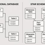
Relational modeling centers on normalization, where entities are broken into distinct tables with keys and relationships. The aim is to eliminate redundancy, enforce data integrity through constraints, and support a wide range of transactional operations. In a typical OLTP design, you will encounter third normal form (3NF) or even higher normalizations, with many small, interrelated tables and frequent writes. The strength of this approach lies in data consistency and update efficiency, particularly in environments with high write throughput and strict referential integrity requirements.
However, the same structural properties that guarantee data accuracy can complicate analytics. Queries may require many joins across dozens of tables, leading to complex SQL, slower performance for large-scale reports, and a heavier burden on ETL processes to denormalize data for BI tools. To illustrate, consider a simplified relational model for a sales domain with customers, orders, products, and order items. The following statements define a minimal, normalized schema that preserves granular history while avoiding data duplication:
CREATE TABLE dim_customer (
  customer_id INT PRIMARY KEY,
  first_name VARCHAR(50),
  last_name VARCHAR(50),
  email VARCHAR(100),
  region VARCHAR(50)
);

CREATE TABLE dim_product (
  product_id INT PRIMARY KEY,
  product_name VARCHAR(100),
  category VARCHAR(50),
  price DECIMAL(10,2)
);

CREATE TABLE order_header (
  order_id INT PRIMARY KEY,
  customer_id INT REFERENCES dim_customer(customer_id),
  order_date DATE,
  status VARCHAR(20)
);

CREATE TABLE order_item (
  order_item_id INT PRIMARY KEY,
  order_id INT REFERENCES order_header(order_id),
  product_id INT REFERENCES dim_product(product_id),
  quantity INT,
  unit_price DECIMAL(10,2)
);
Dimensional Modeling: Star and Snowflake
Dimensional modeling organizes data around a central fact table that captures business events (such as sales transactions) and surrounding dimension tables that describe perspectives for analysis (date, product, customer, store). The star schema keeps dimensions denormalized and directly connected to the fact table based on surrogate keys, resulting in simpler queries and faster scans for typical BI workloads. Snowflake schemas, by contrast, normalize some dimensions into multiple related tables, which can reduce storage but increases join complexity and can require more sophisticated query writing or BI layer logic. The choice between star and snowflake depends on data volumes, user needs, and maintenance capabilities, but for most analytics-centric data warehouses the star schema remains the default starting point.
To illustrate a classic star schema, you define a fact_sales table that records measures such as quantity and total_amount, coupled with several dimension tables that describe the context of each sale. The star design emphasizes a single grain and conformed dimensions so that analytics can be composed consistently across subject areas. The following example shows a simplified star schema and the canonical SQL to create the core tables:
CREATE TABLE dim_date (
  date_id INT PRIMARY KEY,
  calendar_date DATE NOT NULL,
  year INT,
  quarter INT,
  month INT,
  day INT
);

CREATE TABLE dim_product (
  product_id INT PRIMARY KEY,
  product_name VARCHAR(100),
  category VARCHAR(50),
  brand VARCHAR(50)
);

CREATE TABLE dim_customer (
  customer_id INT PRIMARY KEY,
  customer_name VARCHAR(100),
  segment VARCHAR(50),
  region VARCHAR(50)
);

CREATE TABLE dim_store (
  store_id INT PRIMARY KEY,
  store_name VARCHAR(100),
  city VARCHAR(50),
  state VARCHAR(50)
);

CREATE TABLE fact_sales (
  sale_id INT PRIMARY KEY,
  date_id INT REFERENCES dim_date(date_id),
  product_id INT REFERENCES dim_product(product_id),
  customer_id INT REFERENCES dim_customer(customer_id),
  store_id INT REFERENCES dim_store(store_id),
  quantity INT,
  total_amount DECIMAL(12,2)
);
Key Decision Factors: When to Use Each Approach
Choosing between relational and dimensional modeling depends on the primary use cases, data volumes, and the expected workload characteristics. For transactional systems requiring fast, consistent updates and complex referential integrity, a relational model in normalized form is often the best choice. For analytics-first workloads that prioritize straightforward querying, historical analysis, and user-friendly reporting over vast datasets, dimensional models are typically superior. The decision is not binary; most modern data platforms combine approaches, using relational structures for the source systems and dimensional schemas for data warehouses or data marts. The following criteria help frame the decision:
- Analytical latency: How fresh must the analytics be? If near real-time BI is not essential, a dimensional model with periodic ETL is common.
- Query simplicity: Do business users benefit from straightforward joins and predictable grain?
- Data volume and storage: Star schemas can simplify indexing and compression patterns, but snowflake schemas may save space in very large dimension sets.
- Conformity and governance: Are dimensions shared across subject areas (customers, products, dates) and require consistent definitions?
- Change patterns: How often do dimensions change and how to handle slowly changing dimensions (SCD)?
- Maintenance and skills: Does the team prefer denormalized structures with simple BI tooling or normalized designs that emphasize data integrity?
Star Schema Design Principles and Patterns
Adopting a star schema requires deliberate design choices that maximize analytic usability while keeping ETL manageable. Core principles include establishing a single grain for the fact table, designing conformed, stable dimension tables, and implementing sensible slowly changing dimensions. In practice, teams adopt conventions for keying, naming, and granular definitions that enable cross-subject consistency across sales, inventory, and customer analytics. The following patterns frequently emerge in well-governed analytic environments:
- Single fact grain: Each fact table represents one business event at a consistent level of detail, avoiding multiple fact tables at different grains for the same subject area.
- Surrogate keys: Use surrogate integer keys in dimensions to decouple from slow-changing natural keys and to support consistent joins.
- Conformed dimensions: Dimensions such as date and product are shared across multiple fact tables, enabling cross-fact analysis.
- Type 2 SCD for history: When dimension attributes change, preserve historical rows with versioning to support accurate trend analysis.
- Performance-oriented denormalization: Keep dimensions denormalized to reduce the number of joins in typical BI queries.
Performance, Data Quality, and Maintenance
Performance considerations in data warehousing are often the result of query patterns, data volume, and ETL efficiency. Star schemas typically yield faster query performance for analytics because they minimize the number of joins needed to fulfill common queries. However, the benefit depends on proper indexing strategies, partitioning schemes, and the capabilities of the BI tool. Relational models, with normalization, shine in transactional throughput and data integrity but call for careful ETL design to produce analytics-ready representations. A well-governed data platform uses both approaches in complementary roles: source systems rely on relational designs, while the warehouse uses a dimensional model that supports business questions with clarity and speed.
To provide concrete guidance, the following table contrasts OLTP-style relational schemas and OLAP-style dimensional schemas across key dimensions such as query complexity, update operations, and historical support:
| aspect | relational (OLTP) | dimensional (OLAP) |
|---|---|---|
| Query complexity | Complex joins and transactional predicates | Simple, predictable joins to fact table |
| Update operations | High volume inserts/updates with referential integrity | Append-only or bulk-loaded; historical rows preserved |
| Historical data | Often limited, normalized; history requires audit trails | Full history supported through slowly changing dimensions |
Migration, Hybrid Architectures, and Evolution
Modern data platforms rarely rely on a single modeling style for all scenarios. A pragmatic path is to migrate gradually from a purely normalized OLTP-centric design to a dimensional warehouse architecture, while maintaining the source system integrity. Hybrid architectures blend the strengths of both worlds: extract-transform-load processes pull data from relational sources, perform normalization as needed during staging, and load a dimensional model optimized for analytics. When planning such migrations, teams should define clear grains, conformed dimensions, and a staged timeline to minimize disruption and preserve data quality. In practice, you might maintain stable, normalized source systems for accuracy, while building decoupled analytic data marts that mirror business processes with a star or snowflake schema.
Approaches to migration range from re-architecting the data warehouse in waves to more surgical changes, such as creating a new dimensional layer atop existing data marts or adding a metadata-driven virtualization layer. The choice depends on governance, cost, and the ability to maintain backward compatibility with existing reports and dashboards. Regardless of path, maintain a strong emphasis on data lineage, versioned ETL pipelines, and robust validation. Below is a concise outline of steps you might follow in a typical migration project:
- Inventory sources and establish a single, defined grain for the target analytics model.
- Design conformed dimensions and initialize slowly changing dimensions to capture history.
- Implement ETL pipelines that populate the dimensional model while auditing data quality.
- Validate analytics outputs against source reports and establish reconciliation processes.
- Plan for ongoing evolution with versioned schemas and metadata management.
Governance, Metadata, and Stakeholders
Effective data governance is essential for sustainable modeling choices. Clear ownership, defensible naming conventions, and comprehensive metadata about tables, columns, and business definitions help ensure consistent understanding across analysts, engineers, and business users. Dimensional models benefit from explicit data lineage and versioned documentation of conformed dimensions, metrics, and calculated measures. Conversely, relational designs emphasize data integrity and referential constraints that keep transactional data trustworthy. A governance program should cover data quality rules, lineage tracing, and change management to support both OLTP and OLAP pipelines as data moves from source systems to analytics layers.
Successful data teams establish roles such as data stewards, modelers, ETL developers, and BI consumers, all collaborating to maintain alignment between business questions and the underlying structures. Metadata strategies typically include a data catalog, data dictionaries, data lineage visualizations, and automated checks for schema drift. When stakeholders understand the purpose and origin of each dimension and fact, they can trust analytics results and drive better decisions. The right governance model also helps with auditability, regulatory compliance, and ongoing improvement of data models over time.
Practical Lessons and Anti-Patterns
Practitioners frequently encounter recurring patterns—both beneficial and detrimental—when building relational or dimensional warehouses. Common improvements come from enforcing consistent grain, embracing slowly changing dimensions, and adopting conformed dimensions across subject areas. Pitfalls include excessive normalization that complicates analytics, ad-hoc ad-hoc reporting structures that bypass the canonical model, or attempting to force very large denormalized tables into BI tools without considering data governance. By learning from these patterns, teams can reduce rework, lower maintenance costs, and deliver reliable analytics faster. The following considerations help teams stay on the right track:
First, maintain a clear separation between source truth and analytic representations. Treat ETL as a lineage-aware process that preserves data quality while rendering data in the analytic model. Second, design with the user in mind: ensure dimensions and measures reflect business concepts, not just technical artifacts. Third, invest in monitoring and validation so that data quality issues are caught early and do not propagate into dashboards. Finally, avoid overfitting the model to a single reporting tool; build a flexible architecture that supports evolving analytics needs.
Conclusion
Relational and dimensional data models are not rival approaches; they are complementary tools in a data practitioner’s toolkit. The relational perspective ensures data integrity and efficient transactional processing, while the dimensional perspective prioritizes analytics friendliness and user-driven reporting. By recognizing the strengths and limitations of each approach, and by applying a disciplined design process, organizations can build data architectures that scale from operational systems to enterprise-wide analytics. The key is to engineer for clarity, governance, and adaptability, so that data assets remain trustworthy, accessible, and actionable as business questions evolve.
FAQ
What is the primary difference between relational and dimensional data models?
The primary difference lies in the intended use and structural design: relational models emphasize normalization, data integrity, and operational efficiency for transactional systems, while dimensional models emphasize denormalized, user-friendly structures optimized for analytics, reporting, and business intuition. Relational designs support many-to-many, update-heavy workloads; dimensional designs support fast, intuitive queries on historical data through a central fact table and surrounding dimensions.
When should I choose a star schema over a fully normalized relational schema?
Choose a star schema when your primary goals are fast, predictable analytics, simplified SQL for business users, and straightforward aggregation across common dimensions. Star schemas are well-suited for data warehouses and data marts where reporting demands high-performance scans and easy drill-down across time, product, and customer attributes. If you require strict normalization, complex transactional integrity, or highly granular, non-analytic use cases, a fully normalized relational design may be more appropriate, possibly complemented by a dimensional layer for analytics.
How do you handle slowly changing dimensions (SCD) in practice?
Slowly changing dimensions are typically implemented using a combination of surrogate keys, versioned records, and careful ETL logic. The Type 2 approach, which preserves historical rows with new surrogate keys, is common for dimensions where attributes change over time. Other approaches include Type 1 (overwrite) for impermanent attributes, Type 3 (partial history) for limited attribute tracking, and hybrid techniques. The chosen strategy should balance historical fidelity with query simplicity and ETL complexity, guided by business requirements and reporting needs.
What are common anti-patterns to avoid in data modeling?
Common anti-patterns include over-normalization that burdens analytics with excessive joins, under-indexing or poor partitioning that degrade performance, and creating bespoke, isolated data marts that fragment analytics. Another pitfall is treating the analytic model as a moving target to accommodate every new report, which leads to schema drift. Governance gaps—like weak lineage, vague definitions, and inconsistent naming—also undermine trust in analytics. The key is to design with a stable grain, conformed dimensions, and disciplined change management from the outset.